In Credit Assignment in SNNs, we established that training a neural network requires assigning credit to each component: which weight or neuron contributed to an error, and how should they change? For classical neural networks, the backpropagation algorithm solves this by flowing gradients backward through the network. For spiking neural networks, the same idea applies — but with a critical obstacle.
Spiking neurons communicate through discrete, all-or-nothing spikes, described by the Heaviside step function . The derivative of is zero almost everywhere and infinite at the threshold. This means that standard backpropagation produces gradients that are either zero (killing learning) or undefined.
Surrogate gradients solve this problem with a simple trick: keep the Heaviside function during the forward pass, but replace its derivative with a smooth approximation during the backward pass. This chapter explains the idea, derives the math, and walks through a complete training example.
2.2.1The non-differentiability problem
Recall from Point Neuron Models that a spiking neuron emits a spike when its membrane potential exceeds a threshold . We can express this as:
where is the Heaviside step function: it outputs 1 when its argument is positive, and 0 otherwise.
Now consider training a single weight using gradient descent. The loss depends on the spike , which depends on the membrane potential , which depends on the input current . The chain rule gives:
The last two terms are straightforward: , and, if the membrane resistance is set to 1, . The loss derivative depends on the choice of loss function and has an analytical form. But — the derivative of the Heaviside function — is the Dirac delta function:
This evaluates to 0 everywhere except at , where it is undefined (tending to infinity). In practice, this means the gradient is almost always zero, and the weight receives no learning signal. This is known as the non-differentiability problem.
![The Heaviside step function \Theta maps the membrane potential V[t] to a binary spike S[t].
The open circle at V_\text{thr} indicates S[t] = 0 exactly at the threshold; the filled circle indicates S[t] = 1 just above it.](/build/spike_heaviside-ec4e03859e99b287c365e63b033a6fb6.png)
Figure 1:The Heaviside step function maps the membrane potential to a binary spike . The open circle at indicates exactly at the threshold; the filled circle indicates just above it.
2.2.2Surrogate gradient functions
The surrogate gradient approach resolves the non-differentiability problem by decoupling the forward and backward passes:
Forward pass: Use the Heaviside step function as-is. Spikes remain discrete.
Backward pass: Replace the Dirac delta with a smooth surrogate derivative .
This substitution means we are not computing the true gradient of the network — but it turns out that neural networks are remarkably robust to such approximations Neftci et al., 2019.
2.2.2.1The arctangent surrogate
A common choice is the derivative of the arctangent function:
where the left arrow () denotes substitution: we replace the true derivative with this expression during the backward pass. This function is bell-shaped, centered at the threshold, and smoothly decays to zero on either side. Neurons close to the threshold receive the strongest gradient signal, which makes intuitive sense: neurons that are almost spiking are most sensitive to weight changes.
2.2.2.2Other surrogate functions
Many surrogate functions have been proposed. Here are several common choices:
| Name | Surrogate derivative |
|---|---|
| Arctangent | |
| SuperSpike Zenke & Ganguli, 2018 | |
| Fast sigmoid | (SuperSpike with ) |
| Sigmoid | where |
| Rectangular (boxcar) | |
| Triangular |
In practice, the choice of surrogate function has a relatively minor effect on training performance Zenke & Vogels, 2021. What matters more is that the surrogate is smooth, peaked near the threshold, and decays away from it. The choice of surrogate function remains an empirical one, as no theoretical proof establishes which one is the best. Arctangent is a common default due to its smooth, bounded derivative.
2.2.2.3Implementation
The following code implements several surrogate gradient functions and compares them to the true Heaviside derivative:
import numpy as np

def heaviside(v):
    """Forward pass: Heaviside step function."""
    return np.where(v > 0, 1.0, 0.0)

def atan_surrogate(v, alpha=np.pi):
    """Backward pass: arctangent surrogate gradient."""
    return 1.0 / (alpha * (1 + (alpha * v) ** 2))

def superspike_surrogate(v, alpha=100.0):
    """Backward pass: SuperSpike surrogate gradient (Zenke & Ganguli, 2018)."""
    return 1.0 / (alpha * np.abs(v) + 1.0) ** 2

def fast_sigmoid_surrogate(v):
    """Backward pass: fast sigmoid surrogate gradient (SuperSpike with alpha=1)."""
    return 1.0 / (1 + np.abs(v)) ** 2

def sigmoid_surrogate(v):
    """Backward pass: sigmoid surrogate gradient."""
    sig = 1.0 / (1 + np.exp(-v))
    return sig * (1 - sig)

def rectangular_surrogate(v, width=1.0):
    """Backward pass: rectangular (boxcar) surrogate gradient."""
    return np.where(np.abs(v) < width, 0.5 / width, 0.0)

def triangular_surrogate(v):
    """Backward pass: triangular surrogate gradient."""
return np.maximum(0.0, 1.0 - np.abs(v))Solution to Exercise 1 #
The Gaussian surrogate:
def gaussian_surrogate(v):
    return np.exp(-v**2 / 2) / np.sqrt(2 * np.pi)
Compared to the arctangent surrogate, the Gaussian decays much faster away from the threshold (exponential vs. polynomial decay). This means the Gaussian provides gradient signal to a narrower band of neurons around the threshold, which can make training less stable but also more precise. The arctangent has heavier tails and provides a weaker but longer-range gradient signal.
2.2.3The neuron as a filter: from the SRM to a training model
Before we can train a spiking neural network, we need to understand how gradient information flows through time. A spiking neuron is a recurrent system: its state at time depends on its state at time .
The Spike Response Model decomposes a neuron into linear filters followed by a threshold nonlinearity Gerstner et al., 2014. The membrane potential is a sum of two convolutions: input filtered through the membrane kernel , plus the spike afterpotential that captures reset and refractoriness after each output spike. The only nonlinearity is the threshold crossing that produces a spike.
This decomposition is exactly what makes surrogate gradients principled: the filters and are already differentiable, so we only need to approximate the derivative of one nonlinearity — the Heaviside function at the threshold.
2.2.3.1The simplified LIF neuron
The full neuron derived in Section 1.1.2.2 has several hyperparameters (, , ). For deep learning, we simplify this by introducing the decay rate , which collapses the time constant into a single parameter. Starting from the discrete equation and setting and :
where is the voltage decay from Section 1.1.2.2. A value of close to 1 means slow decay (long memory); close to 0 means fast decay.
The input current is now weighted by a learnable parameter , absorbing the effect of the membrane resistance. The complete simplified neuron model becomes:
In the language of the SRM, the decay term implements the membrane filter (exponential integration of past inputs), while the reset term implements the spike afterpotential (reset by subtraction). The only free hyperparameter is .
2.2.3.2Unrolling through time
Equation (8) describes a recurrence: depends on , which depends on , and so on. We can visualize this by unrolling the computation graph across time steps:
![Recurrent representation of spiking neurons.
(a) A spiking neuron with implicit recurrence (\beta, membrane decay) and explicit recurrence (the feedback path from the output spike back into the membrane).
(b) The equivalent spiking neuron illustrated as an unrolled computational graph across time steps t=0,1,2 (explicit recurrence omitted); \beta connections carry the membrane V[t] forward, W injects the input I_\text{in}[t], and -V_\text{thr} is the reset term subtracted from the membrane after each output spike S_\text{out}[t].](/build/unrolled_lif-3849a1bc5c95949b8a3b00f6f3bf7ba9.png)
Figure 2:Recurrent representation of spiking neurons. (a) A spiking neuron with implicit recurrence (, membrane decay) and explicit recurrence (the feedback path from the output spike back into the membrane). (b) The equivalent spiking neuron illustrated as an unrolled computational graph across time steps (explicit recurrence omitted); connections carry the membrane forward, injects the input , and is the reset term subtracted from the membrane after each output spike .
Each column represents one time step. The horizontal connections (weighted by ) represent the membrane potential decay. The vertical connections (weighted by ) represent the synaptic input. The connection weighted by represents the reset mechanism.
This unrolled graph looks just like a deep feedforward network — except that the weight is shared across all time steps. This observation is the key insight that connects SNN training to recurrent neural network training.
2.2.3.3Backpropagation through time
To train this network, we apply backpropagation through time (BPTT). The weight influences the loss at every time step, so the total gradient is a sum over all time steps:
The constraint enforces causality: we consider the contributions of only for past and present inputs. Because is shared across time (), a change to at any step affects all steps equally.
Consider the contribution from one step back, :
The temporal derivative comes directly from Eq (8). In the SRM figure, this is the derivative through the membrane filter — it is exact, not approximated. The surrogate only enters at the term, i.e., the threshold crossing. Going further back in time, each additional step multiplies the current value by another factor of , so the gradient contribution from steps in the past is proportional to . Since , contributions from the distant past decay exponentially — which is why the choice of matters.
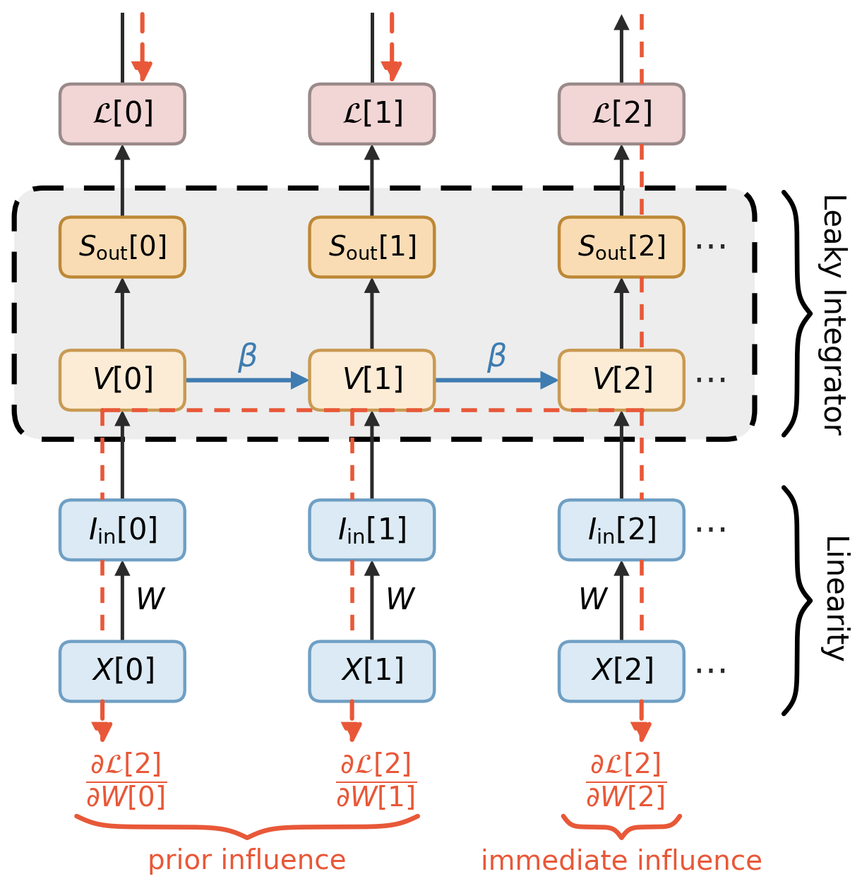
Figure 3:Backpropagation through time (BPTT) for the unrolled LIF neuron. Solid arrows show the forward pass; dashed orange arrows show the gradient flowing backward through time. Gradients of earlier time steps (prior influence) require more steps of backward propagation, each multiplying by .
2.2.3.4Implementation
The code below shows how to implement the same neuron with surrogate gradient support across three frameworks. In each case, the forward pass computes the true Heaviside step and the backward pass replaces its derivative with a surrogate:
import numpy as np

class LIFNeuron:
    """A single LIF neuron with surrogate gradient support."""

    def __init__(self, beta=0.9, threshold=1.0):
        self.beta = beta
        self.threshold = threshold

    def forward(self, inputs, num_steps):
        """Run the neuron for num_steps, recording states for backprop.

        Args:
            inputs: array of shape (num_steps,), weighted input current WX[t]
            num_steps: number of simulation time steps

        Returns:
            spikes: array of shape (num_steps,), output spikes
            membrane: array of shape (num_steps,), membrane potential
        """
        mem = 0.0
        spikes = np.zeros(num_steps)
        membrane = np.zeros(num_steps)

        for t in range(num_steps):
            mem = self.beta * mem + inputs[t] - spikes[t - 1] * self.threshold if t > 0 else inputs[t]
            spikes[t] = 1.0 if mem > self.threshold else 0.0
            membrane[t] = mem

        return spikes, membrane

    def surrogate_grad(self, membrane):
        """Arctangent surrogate gradient - called manually in the backward pass.

        Args:
            membrane: array of shape (num_steps,), membrane potential values

        Returns:
            grads: array of shape (num_steps,), surrogate gradient dS/dV
        """
        v = membrane - self.threshold
        return 1.0 / (np.pi * (1 + (np.pi * v) ** 2))
import torch
import torch.nn as nn
class SpikeFunction(torch.autograd.Function):
"""Heaviside forward pass; arctangent surrogate in the backward pass.
Subclassing torch.autograd.Function lets PyTorch's autograd engine
call our custom backward whenever .backward() flows through a spike.
"""
@staticmethod
def forward(ctx, v, threshold):
ctx.save_for_backward(v - threshold)
return (v > threshold).float()
@staticmethod
def backward(ctx, grad_output):
(v_shifted,) = ctx.saved_tensors
surrogate = 1.0 / (torch.pi * (1 + (torch.pi * v_shifted) ** 2))
return grad_output * surrogate, None
class LIFNeuron(nn.Module):
def __init__(self, beta=0.9, threshold=1.0):
super().__init__()
self.beta = beta
self.threshold = threshold
def forward(self, inputs):
"""
Args:
inputs: tensor of shape (num_steps, ...)
Returns:
spikes: tensor of shape (num_steps, ...)
"""
mem = torch.zeros_like(inputs[0])
spike_list = []
for inp in inputs:
mem = self.beta * mem + inp
spk = SpikeFunction.apply(mem, self.threshold)
mem = mem - spk * self.threshold
spike_list.append(spk)
return torch.stack(spike_list)import jax
import jax.numpy as jnp
@jax.custom_vjp
def spike_fn(v, threshold):
"""Heaviside forward pass; arctangent surrogate in the backward pass.
jax.custom_vjp lets us define the vector-Jacobian product (VJP)
separately from the forward computation, so jax.grad flows through
our surrogate instead of the true (undefined) Heaviside derivative.
"""
return jnp.where(v > threshold, 1.0, 0.0)
def spike_fn_fwd(v, threshold):
return spike_fn(v, threshold), (v - threshold,)
def spike_fn_bwd(res, g):
(v_shifted,) = res
surrogate = 1.0 / (jnp.pi * (1 + (jnp.pi * v_shifted) ** 2))
return g * surrogate, None
spike_fn.defvjp(spike_fn_fwd, spike_fn_bwd)
def lif_step(mem, inp, beta, threshold):
"""Single LIF time step - differentiable via spike_fn above."""
mem = beta * mem + inp
spk = spike_fn(mem, threshold)
mem = mem - spk * threshold
return spk, mem2.2.4Loss functions and output decoding
Before we can train a network, we need to define what “correct” means. In a spiking neural network, the output neurons produce spike trains — sequences of 0s and 1s over time. We need a way to interpret these spike trains as predictions and compare them to targets.
2.2.4.1Rate coding
The most common approach for classification is rate coding (see Rate Encoding): the predicted class is the output neuron with the highest total spike count (or equivalently, the highest firing rate) over the simulation:
This is analogous to taking the neuron with the highest activation in a classical neural network.
2.2.4.2Cross-entropy loss on the membrane potential
To create a differentiable loss, we apply the cross-entropy loss to the membrane potential rather than to the discrete spikes. The softmax of the membrane potential for output classes gives:
The cross-entropy between and the one-hot target is:
The effect is that the membrane potential of the correct class is encouraged to stay above the threshold (producing spikes), while incorrect classes are suppressed below the threshold.
2.2.4.3Summing over time
Since the network runs for time steps, we compute the loss at every step and sum:
This is the objective that BPTT differentiates through, as described in Eq (9).
2.2.5Putting it together: training on MNIST
We now have all the pieces to train a spiking neural network:
A simplified neuron (Eq (8))
Surrogate gradients to handle non-differentiable spikes (Eq (5))
BPTT to propagate gradients through time (Eq (9))
A loss function applied at every time step (Eq (14))
Let’s put this together and train a feedforward SNN on the MNIST handwritten digit dataset.
2.2.5.1Network architecture
We build a two-layer fully connected spiking neural network:
Input: 784 neurons (2828 pixel images, flattened)
Hidden layer: 1000 neurons
Output layer: 10 neurons (one per digit class)
The same static input image is presented at every time step for steps, giving the network time to integrate and produce spikes.
import numpy as np

def softmax(x):
    """Numerically stable softmax."""
    e_x = np.exp(x - np.max(x, axis=-1, keepdims=True))
    return e_x / e_x.sum(axis=-1, keepdims=True)

def cross_entropy_loss(logits, targets):
    """Cross-entropy loss.

    Args:
        logits: array of shape (batch_size, num_classes)
        targets: array of shape (batch_size,), integer class labels

    Returns:
        loss: scalar, mean cross-entropy loss
        d_logits: array of shape (batch_size, num_classes), gradient of loss w.r.t. logits
    """
    probs = softmax(logits)
    batch_size = logits.shape[0]
    loss = -np.log(probs[np.arange(batch_size), targets] + 1e-8).mean()
    d_logits = probs.copy()
    d_logits[np.arange(batch_size), targets] -= 1.0
    d_logits /= batch_size
return loss, d_logits2.2.5.2Forward pass
The forward pass simulates the network over time steps, storing intermediate values needed for the backward pass:
def forward(x, W1, W2, beta, threshold, num_steps):
    """Forward pass of a two-layer SNN.

    Args:
        x: input array of shape (batch_size, 784)
        W1: weights of shape (784, 1000)
        W2: weights of shape (1000, 10)
        beta: membrane decay rate
        threshold: spike threshold
        num_steps: number of simulation time steps

    Returns:
        cache: dict of intermediate values for the backward pass
    """
    batch_size = x.shape[0]

    # Hidden layer state
    mem1 = np.zeros((batch_size, 1000))
    spk1 = np.zeros((batch_size, 1000))

    # Output layer state
    mem2 = np.zeros((batch_size, 10))
    spk2 = np.zeros((batch_size, 10))

    # Storage for backprop
    mem1_rec, spk1_rec = [], []
    mem2_rec, spk2_rec = [], []

    for t in range(num_steps):
        # Layer 1: input -> hidden
        cur1 = x @ W1                                      # synaptic current
        mem1 = beta * mem1 + cur1 - spk1 * threshold       # membrane update
        spk1 = (mem1 > threshold).astype(np.float64)        # spike

        # Layer 2: hidden -> output
        cur2 = spk1 @ W2                                    # synaptic current
        mem2 = beta * mem2 + cur2 - spk2 * threshold        # membrane update
        spk2 = (mem2 > threshold).astype(np.float64)         # spike

        mem1_rec.append(mem1)
        spk1_rec.append(spk1)
        mem2_rec.append(mem2)
        spk2_rec.append(spk2)

    cache = {
        'x': x,
        'mem1': np.stack(mem1_rec),   # (T, batch, 1000)
        'spk1': np.stack(spk1_rec),   # (T, batch, 1000)
        'mem2': np.stack(mem2_rec),    # (T, batch, 10)
        'spk2': np.stack(spk2_rec),   # (T, batch, 10)
    }
return cache2.2.5.3Backward pass with surrogate gradients
The backward pass flows gradients back through the states for each time step, using the arctangent surrogate in place of the Heaviside derivative:
def backward(cache, targets, W1, W2, beta, threshold, num_steps):
    """Backward pass using BPTT with surrogate gradients.

    Args:
        cache: dict from forward pass
        targets: array of shape (batch_size,), integer class labels
        W1, W2: weight matrices
        beta, threshold: neuron parameters
        num_steps: number of time steps

    Returns:
        dW1, dW2: gradients for the weight matrices
        total_loss: scalar loss summed over time
    """
    mem1_rec = cache['mem1']
    spk1_rec = cache['spk1']
    mem2_rec = cache['mem2']
    x = cache['x']

    dW1 = np.zeros_like(W1)
    dW2 = np.zeros_like(W2)
    total_loss = 0.0

    # Gradient flowing back into the membrane potential from future time steps
    d_mem2_future = np.zeros_like(mem2_rec[0])
    d_mem1_future = np.zeros_like(mem1_rec[0])

    for t in reversed(range(num_steps)):
        # --- Output layer loss ---
        loss_t, d_logits = cross_entropy_loss(mem2_rec[t], targets)
        total_loss += loss_t

        # Gradient into mem2: from the loss + from future time steps (decay)
        d_mem2 = d_logits + d_mem2_future

        # Surrogate gradient: dS/dV for the output layer
        v2 = mem2_rec[t] - threshold
        sg2 = 1.0 / (np.pi * (1 + (np.pi * v2) ** 2))

        # Gradient through spike -> weight2
        d_spk2 = d_mem2 * sg2  # not used further here, but would be for deeper nets

        # dW2: Matrix multiplication of spk1^T and d_mem2 (input to layer 2 is spk1)
        dW2 += spk1_rec[t].T @ d_mem2

        # Propagate the gradient back to spk1
        d_spk1_from_layer2 = d_mem2 @ W2.T

        # Surrogate gradient: dS/dV for the hidden layer
        v1 = mem1_rec[t] - threshold
        sg1 = 1.0 / (np.pi * (1 + (np.pi * v1) ** 2))

        # Gradient into mem1: from layer2 (through the surrogate) + from future time steps
        d_mem1 = d_spk1_from_layer2 * sg1 + d_mem1_future

        # dW1: Matrix multiplication of x^T and d_mem1
        dW1 += x.T @ d_mem1

        # Propagate the membrane gradient back in time (decay connection)
        d_mem2_future = d_mem2 * beta
        d_mem1_future = d_mem1 * beta

return dW1, dW2, total_loss2.2.5.4Training loop
With the forward and backward passes defined, the training loop follows the standard pattern: iterate over batches, compute the loss, calculate gradients, and update weights:
def train(train_images, train_labels, num_epochs=1, batch_size=128,
          lr=5e-4, beta=0.95, threshold=1.0, num_steps=25):
    """Train a two-layer SNN on image classification.

    Args:
        train_images: array of shape (N, 784), flattened images
        train_labels: array of shape (N,), integer labels
        num_epochs: number of training epochs
        batch_size: mini-batch size
        lr: learning rate
        beta: membrane decay rate
        threshold: spike threshold
        num_steps: simulation time steps

    Returns:
        W1, W2: trained weight matrices
        loss_history: list of loss values
    """
    num_samples = train_images.shape[0]

    # Initialize all weights (Xavier initialization)
    W1 = np.random.randn(784, 1000) * np.sqrt(2.0 / 784)
    W2 = np.random.randn(1000, 10) * np.sqrt(2.0 / 1000)

    loss_history = []

    for epoch in range(num_epochs):
        # Shuffle the data
        perm = np.random.permutation(num_samples)
        train_images = train_images[perm]
        train_labels = train_labels[perm]

        for i in range(0, num_samples, batch_size):
            x_batch = train_images[i:i + batch_size]
            y_batch = train_labels[i:i + batch_size]

            # Forward
            cache = forward(x_batch, W1, W2, beta, threshold, num_steps)

            # Backward
            dW1, dW2, loss = backward(
                cache, y_batch, W1, W2, beta, threshold, num_steps
            )

            # Update weights (gradient descent)
            W1 -= lr * dW1
            W2 -= lr * dW2

            loss_history.append(loss)

return W1, W2, loss_historySolution to Exercise 2 #
def evaluate(test_images, test_labels, W1, W2, beta, threshold, num_steps):
    cache = forward(test_images, W1, W2, beta, threshold, num_steps)
    # Sum spikes over time for each output neuron
    spike_counts = cache['spk2'].sum(axis=0)  # (N, 10)
    predictions = spike_counts.argmax(axis=1)
    accuracy = (predictions == test_labels).mean()
    return accuracy
Higher (e.g. 0.95–0.99) typically gives better accuracy because the neuron retains more information across time steps, effectively integrating over a longer time window. Lower (e.g. 0.5) causes the membrane potential to decay quickly, making it harder for the neuron to accumulate enough charge to spike meaningfully. However, very high can also result in slow convergence because the reset mechanism becomes less effective.
2.2.6When to use surrogate gradients
Surrogate gradient training is the most widely used method for training SNNs today. It is well suited when:
Accuracy is the priority: Surrogate gradients leverage the full power of gradient-based optimization, typically outperforming non-gradient-based SNN training methods, though exact-gradient approaches can match or exceed them at greater computational cost
Offline training is acceptable: Training happens in batch mode on a GPU, not on the target hardware
A teaching signal is available: Labels, self-supervised targets, or any other differentiable loss signal can be used — surrogate gradients aren’t limited to strictly supervised setups
More complex neuron models: The SRM perspective shows that surrogate gradients work for any neuron model more complex than the simple LIF, as long as it decomposes into linear filters plus a threshold — including adaptive neurons with multiple spike afterpotential kernels , or neurons with synaptic current dynamics
The main limitations are:
Memory cost: Full BPTT requires storing intermediate states for all time steps (though truncated BPTT and gradient checkpointing can help)
Not biologically plausible: The backward pass requires symmetric weights and global error signals — mechanisms not found in biological neural circuits
Offline only: The network cannot adapt during deployment; training and inference are separate phases
Alternatives that address some of these limitations — exact-gradient methods, biologically plausible learning rules, and meta-learning approaches that improve the learning process itself — are covered in chapters planned for a later release.
2.2.7Related reading
Here is a list of resources sorted by topic (please help expand the list):
Foundational: Neftci et al., 2019, Zenke & Ganguli, 2018, Eshraghian et al., 2023
SRM and filter perspective: Gerstner et al., 2014 (Ch. 1, 6)
Surrogate function comparisons: Zenke & Vogels, 2021
BPTT for SNNs: Werbos, 1990, Bellec et al., 2018
Applications: Bellec et al., 2020
Cite this chapter
Kembay, Assel; Eshraghian, Jason; Pedersen, Jens Egholm (2026). Surrogate Gradient Training. In Gaurav, Ramashish; Pedersen, Jens Egholm; Bogdan, Petrut (Eds.), Practical Spiking Neural Networks. Version 0.8. Open Neuromorphic. https://snnbook.net/topics/2_2_surrogate_gradients
@incollection{snnbook2026-surrogate-gradients,
  author    = {Kembay, Assel and Eshraghian, Jason and Pedersen, Jens Egholm},
  title     = {{Surrogate Gradient Training}},
  booktitle = {{Practical Spiking Neural Networks}},
  editor    = {Gaurav, Ramashish and Pedersen, Jens Egholm and Bogdan, Petrut},
  publisher = {Open Neuromorphic},
  year      = {2026},
  edition   = {Version 0.8},
  url       = {https://snnbook.net/topics/2_2_surrogate_gradients},
}- Neftci, E. O., Mostafa, H., & Zenke, F. (2019). Surrogate Gradient Learning in Spiking Neural Networks: Bringing the Power of Gradient-based optimization to spiking neural networks. IEEE Signal Processing Magazine, 36(6), 51–63. 10.1109/MSP.2019.2931595
- Zenke, F., & Ganguli, S. (2018). SuperSpike: Supervised Learning in Multilayer Spiking Neural Networks. Neural Computation, 30(6), 1514–1541. 10.1162/neco_a_01086
- Zenke, F., & Vogels, T. P. (2021). The Remarkable Robustness of Surrogate Gradient Learning for Instilling Complex Function in Spiking Neural Networks. Neural Computation, 33(4), 899–925. 10.1162/neco_a_01367
- Gerstner, W., Kistler, W. M., Naud, R., & Paninski, L. (2014). Neuronal dynamics: From single neurons to networks and models of cognition. Cambridge University Press.
- Eshraghian, J. K., Ward, M., Neftci, E. O., Wang, X., Lenz, G., Dwivedi, G., Bennamoun, M., Jeong, D. S., & Lu, W. D. (2023). Training Spiking Neural Networks Using Lessons From Deep Learning. Proceedings of the IEEE, 111(9), 1016–1054. 10.1109/JPROC.2023.3308088
- Werbos, P. J. (1990). Backpropagation Through Time: What It Does and How to Do It. Proceedings of the IEEE, 78(10), 1550–1560. 10.1109/5.58337
- Bellec, G., Salaj, D., Subramoney, A., Legenstein, R., & Maass, W. (2018). Long short-term memory and learning-to-learn in networks of spiking neurons. Advances in Neural Information Processing Systems, 31.
- Bellec, G., Scherr, F., Subramoney, A., Hajek, E., Salaj, D., Legenstein, R., & Maass, W. (2020). A Solution to the Learning Dilemma for Recurrent Networks of Spiking Neurons. Nature Communications, 11(1), 3625. 10.1038/s41467-020-17236-y