This topic covers training SNNs end to end: from tracing errors back to the parameters that caused them, to building practical and efficient setups for your use case.
Why Training Matters
The previous topic, Foundations of SNNs, identifies the core elements of Spiking Neural Networks. But, then what? Randomly putting spiking neurons together is rarely useful. The connections, time constants, and thresholds need to adapt to a specific scenario: we need to train the parameters of the network to achieve the desired behavior. This is what we cover in this topic.
To make this concrete, here is a small before-and-after experiment.
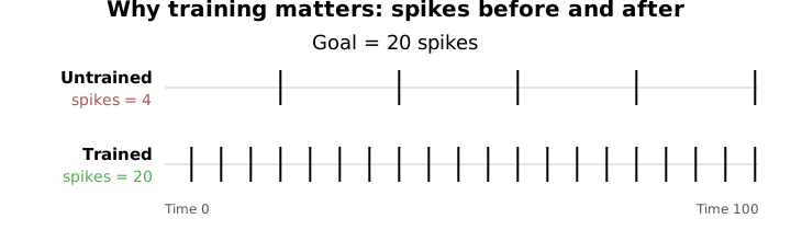
Figure 1:An Integrate-and-Fire neuron before (top) and after (bottom) training. With a poor initial weight it fires too little. After adjusting the single weight, we reach the goal of 20 spikes. The point of this topic is to show you different ways to go from an untrained to a trained network.
We use the simplest possible spiking neuron: a single Integrate-and-Fire (IF) unit (see Foundations of SNNs) driven by a constant input that it scales by one weight .Our goal is modest — make the neuron fire at a target rate. With a poor initial , the firing rate is wrong; training nudges until the firing rate matches the target.
You might object that you can calculate the optimal set of parameters from the beginning. That you know the exact solution your system needs to adhere to, so you have no need to modify the network afterwards. If that is the case, you can skip this topic on training entirely and continue to the topic on Deploying SNNs. But please tell us the secret behind your approach!
We write about training because it is generally harder in SNNs for two reasons: recurrence (in time) and discontinuities (spikes). Classical neural networks usually feature continuous activation functions that are easily differentiable, but spiking neurons are state-dependent nonlinearities that unroll in time, which makes them expensive to compute. Furthermore, the activations have jumps that are challenging to differentiate. Luckily, there are a number of ideas and methods to get around these problems, which we present in this topic.
Background
If you think about a neural network as a system of equations, the search for good, even optimal, solutions reduces to a simple optimization process. Imagine a simple linear system where some vector output is produced by multiplying a matrix with some input vector .
Here, and are given, so we can solve for directly.
In a neural network, however, is unknown. Additionally, imagine that our network has nonlinearities, the above equation quickly becomes unwieldy. This gets even worse when we realize that the nonlinearities can have parameters such as conductivity and resistivity (see the chapter on Point Neuron Models)! In fact, neural networks are so unwieldy that a famous textbook on nonlinear systems calls them a “frontier” (see Table 1), in contrast to other things like linear oscillators and pendulum dynamics.
Table 1:Classification of dynamical systems by linearity and number of variables (). Adapted from Strogatz (2019).
| Linear | Nonlinear | |
|---|---|---|
| Growth, decay, or equilibrium | Bifurcations Fixed points | |
| Linear oscillator Mass and spring | Pendulum Limit cycles | |
| Electrical engineering Multi-variable systems | 3-body problem Forced nonlinear oscillators | |
| Coupled harmonic oscillators Solid-state physics | Coupled nonlinear oscillators Neural networks |
Given that we cannot solve the problem directly, we have to search for a solution. One way to approach this is to define a measure of “badness”: how “bad” is the current network? That is useful because we can start asking how we can make the network less “bad”. Training is simply reducing that “badness” over time, and when we hit 0, we are done. In machine learning, that “badness” is called “loss”, and it is usually denoted as :
Here our loss is the distance between the network applied to the input (the network prediction) on one hand, and the expected/desired value on the other. Thus, training means changing the parameters so that the distance becomes smaller and smaller, that is, moves closer and closer to the goal.
If you took calculus in high school you might realize that we want to change in the direction of a downward slope: we want the change of to give us smaller errors. This is known as the gradient of , written as . We are interested in the negative of this gradient () because we want to decrease, at shown in Figure 2.
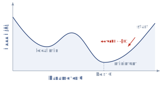
Figure 2:The loss drawn as a landscape over the parameters . Training starts somewhere on a slope and moves downhill toward a minimum.
We can minimize the error by using a distance metric, such as the loss, as shown in Figure 2. But there is a catch: we might be unlucky and land in local minima which look like optimal solutions because the gradient is zero, but can, in fact, be terrible solutions.
Local minima are not the only hazard while training neural networks, and it turns out that spiking networks are much harder to train than classical networks for two reasons: The first is time: an SNN unrolls its computation over many timesteps, so a single step downhill has to account for how a parameter shaped the output at every timestep, not just one. The second is discontinuity: a spike is an abrupt jump, a cliff in the landscape rather than a gentle curve, and at a cliff, the gradient we just leaned on, is undefined! Where a classical network hands us a smooth surface to descend, an SNN hands us a jagged one that also stretches out in time. If this is unclear, the chapter on Credit Assignment in SNNs explains this in detail.
The rest of this topic is, in essence, about different ways to effectively navigate this loss landscape.
Contents of this Topic
The topic is organized around methods for solving the credit assignment problem for SNNs: determining which parameters are responsible for the network’s error, both in space and time. We begin by discussing gradient methods in the chapter on Surrogate Gradient Training because they closely resemble well-established methods in neural networks and because they are popular in the present-day SNN literature.
Here is the list of chapters in this release:
Credit Assignment: How do you attribute success or failure to specific network components when dealing with both spatial connectivity and temporal dynamics? This chapter explores the fundamental challenge of credit assignment in SNNs, including backpropagation through time for spiking networks.
Surrogate Gradients: How can we train spiking neurons despite being non-differentiable? This chapter introduces surrogate gradient methods that approximate gradients during the backward pass while maintaining spike-based computation in the forward pass.
Planned for later releases
Further chapters are in preparation and will appear in later releases. They cover exact gradients, which exploit precise spike timing rather than approximating the threshold; meta learning, which improves the learning mechanism itself, a process known as ‘learning to learn’; biologically inspired and evolutionary methods, which abandon the comfortable realm of backpropagation for algorithms that are decentralized, asynchronous, and buildable exclusively from components in the Topic on Foundations of SNNs; ANN-to-SNN conversion, which circumvents the training problem by training a classical network before converting it; and training optimization, which addresses accuracy and speed for memory- and compute-intensive training algorithms.
Cite this chapter
Gaurav, Ramashish; Pedersen, Jens Egholm; Bogdan, Petrut (2026). Training SNNs. In Practical Spiking Neural Networks. Version 0.8. Open Neuromorphic. https://snnbook.net/topics/2_training
@incollection{snnbook2026-training,
  author    = {Gaurav, Ramashish and Pedersen, Jens Egholm and Bogdan, Petrut},
  title     = {{Training SNNs}},
  booktitle = {{Practical Spiking Neural Networks}},
  publisher = {Open Neuromorphic},
  year      = {2026},
  edition   = {Version 0.8},
  url       = {https://snnbook.net/topics/2_training},
}- Strogatz, S. H. (2019). Nonlinear Dynamics and Chaos: With Applications to Physics, Biology, Chemistry, and Engineering (2nd ed.). CRC Press. 10.1201/9780429492563