To improve any neural network, we need to solve the credit assignment challenge: when the network makes an error, how do we determine which components to adjust? And by how much? This chapter explains the intuition and mathematics behind credit assignment with an emphasis on time because, unfortunately, credit assignment becomes harder when you work with stateful neurons and networks, which are described in the previous topic on Foundations of SNNs.
2.1.1The Credit Assignment Problem
The core question in this chapter is: Given an output error, which neurons and synapses contributed to that error? The term credit assignment was coined by Marvin Minsky in a 1960 paper Minsky, 1961, but he went the other way around: how do we reward the good parts of the network. Whether you think about credit as “reward” or “punishment”, the essence of the problem is the same:
The credit for a working program can only be assigned to [...] subroutines, and as these operate in hierarchies we should not expect individual instruction reinforcement to work well. - Minsky (1961)
What Minsky is saying, is that our networks consist of subcomponents that, together, make up the whole. So, if we are to assign credit and improve the network, we first need to understand how each component contributes to the whole. What is the contribution of, say, a synapse to the network output? Only when we understand that contribution, do we know how to change the synapse. That is the fundamental problem of credit assignment: how do we assign credit to the individual components?
2.1.1.1Credit assignment in space
The structural credit assignment problem is to determine which internal decisions are responsible - Minsky (1961)
In a feedforward network, credit assignment reduces to a structural question: which connections along the path from input to output are responsible for the error?
Consider a single linear layer with a single weight, and no bias term, as shown in Figure 1. Following the example in the figure, the layer receives some input (1), and the objective is to output 2. In this example, is set to , so the output is off by one. We can solve this by adjusting the linear weight from , which gives : we’ve reached our goal!
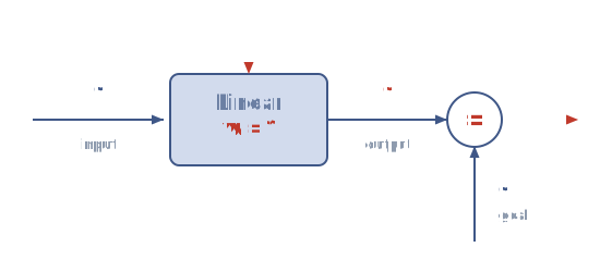
Figure 1:Spatial credit assignment. A linear weight gets readjusted from to ensure that the output is the same as the goal: 1.
Now, consider the case shown in Figure 2, where we have two linear layers, both with , and a goal of . The output becomes , since and . Our error is now , but which parts of the network do we update? And by how much? The simplest solution would probably be to set or to , but there are many more solutions.
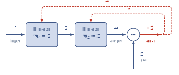
Figure 2:Spatial credit assignment with two layers. Which layer should receive the update? With multiple components, this becomes less clear.
Solution to Exercise 1 #
We could set and , which yields and .
In general, we need to solve the equation . But we have more than one variable, so there are infinitely many solutions! This is why credit assignment is hard.
Even in this minimal example, there is no single correct answer: many combinations of weights produce the same output. This ambiguity is at the heart of spatial credit assignment, and it only grows worse as networks get deeper and more complex. A caveat on the word ambiguity: that many weight settings solve the task does not make credit undefined. Given a loss, the gradient still prescribes one well-defined update. It is the solution set, not the credit signal, that is degenerate: many distinct weight settings collapse onto the same output, so the task alone singles out none of them. Now, imagine adding time to the equation.
2.1.1.2Credit assignment in time
In networks without memory, credit assignment only needs to trace errors backward through layers. But neurons with state carry information across time, and a spike at timestep may cause an error at timestep . Now we must assign credit not just to the right component, but to the right component at the right moment.
To see why, take the single-weight example from Figure 1 and unroll it in time: the same neuron, with the same weight , but now using state. Acting at and again at carries state forward from one step to the next (Figure 3). Notice that this is the same picture as the two-layer case in Figure 2, only now the “depth” is time rather than space. The output is wrong by the same amount, and the same question returns: which timestep should receive the update?
The catch is that is shared: the very same parameter acts at every timestep. When we ask how a small change in affects the final error, the answer is not a single number but a sum: one contribution from the role played at , another from its role at , and so on for every step it was active. Unrolling the network in time and differentiating makes this explicit:
This is exactly the backpropagation through time (BPTT) computation Werbos, 1990: we unroll the recurrence into a deep feedforward graph, one layer per timestep, and propagate the error backward through it.
Bundling every moment into a single gradient is convenient for computing an update, but it hides the same ambiguity we met in space. The total error could be blamed on what the neuron did at , on what it did at , or split between the two in any proportion; the sum in (1) constrains only the whole, never the per-step shares. Where the spatial two-layer case had infinitely many pairs that yield the same output, the temporal case has infinitely many ways to distribute one shared weight’s error across the moments it acted. Time, in other words, is just another axis of depth - and credit assignment is ambiguous along it for exactly the same reason.
Figure 3:Temporal credit assignment. The same neuron (weight ) acts at and , carrying its state forward. The output is off by the same error as the two-layer case, and the dashed feedback shows the ambiguity: which timestep should receive the update? As with multiple spatial weights, there are infinitely many solutions.
The gradient in (1) really flows through the chain of state updates . Carrying the membrane potential step by step through the entire chain of state updates makes SNNs especially hard:
Non-differentiable spikes: the spike threshold has zero gradient almost everywhere, blocking the chain rule exactly where information is sent.
Vanishing or exploding gradients: errors travel through a long product of state terms, arriving faint or wildly amplified.
Sparse, nonlinear dynamics: only some neurons spike, and small changes can have large, delayed downstream effects.
2.1.1.3Credit assignment parameter updates
Once we know which components contributed to an error, we face a second question: how do we translate that knowledge into concrete parameter changes?
The geometry of the gradients: natural and isometric gradients
Knowing which component to blame tells us the direction to move a parameter, but not how far. And distance is subtle: a step of 0.1 in one weight may barely change the network’s behavior, while the same step in another may ruin it. Parameters live on different scales, so measuring an update by raw parameter distance (as plain gradient descent does) treats unlike things alike.
This matters even when credit is assigned perfectly. A vanilla gradient step scales every parameter by the same learning rate, so it over-corrects the components the loss is very sensitive to and under-corrects those it is nearly flat in. The direction can be right while the magnitude is wrong.
The natural gradient Amari, 1998 addresses this by measuring distance in the space of the network’s outputs rather than its parameters. It rescales the update by the Fisher information metric, so a unit step means “change the output distribution by this much”, regardless of how the network is parameterized. The update becomes invariant to reparameterizations.
For SNNs the point is sharper still. State and time warp the loss landscape: the same weight enters the loss at many timesteps (see Figure 3), so its effective curvature compounds over the sequence. A metric-aware (or isometric, distance-preserving) update ensures steps are taken equally in both space and time, rather than letting early timesteps or “loud” neurons dominate.
2.1.1.4A note on scalability
The ambiguity we have discussed so far is a question of correctness: which component, at which moment, deserves the credit. Scalability is a separate, practical question: even when we know how to compute the credit, can we afford to?
Backpropagation through time answers the credit question by unrolling the network into one layer per timestep and storing every intermediate state, so it can later walk the errors backward. That storage is the bottleneck. Memory grows with the sequence length multiplied by the size of the network, because every activation along the way must be kept until the backward pass reaches it; compute grows with the same product, since each stored step must also be revisited. A long recording or a deeply recurrent loop can exhaust memory long before the method itself runs into any limit.
This cost is a large part of why the coming chapters exist. It motivates truncating the unroll to a short window, propagating sensitivities forward in time instead of backward (real-time recurrent learning (RTRL), which stores nothing extra as the sequence grows but scales poorly in network size Marschall et al., 2020) or abandoning the global backward pass entirely in favor of local rules (such as eligibility traces, plasticity, and reward signals) that update each synapse from information it already has on hand. Correctness tells us what credit assignment should compute. Scalability decides which approximation we can actually run.
2.1.1.5Why not just use backpropagation?
Beyond its memory cost, BPTT sits awkwardly with biology and neuromorphic hardware Lillicrap et al., 2020: the backward pass needs the transpose of the forward weights (the weight-transport problem), it requires separate locked forward and backward phases, and its updates are non-local. These objections motivate the alternatives that follow, some of which keep backprop’s form but swap the transposed weights for fixed random ones (feedback alignment Lillicrap et al., 2016, direct feedback alignment Nøkland, 2016) while others drop the global backward pass entirely.
2.1.2Approaches to solving credit assignment
The rest of this topic explores three families of approaches, each developed fully in the chapters that follow:
Gradient-based: approximate the derivatives and flow error signals backward, just as in classical deep learning (Surrogate Gradient Training).
Eligibility-based: each synapse keeps a running eligibility trace of its recent activity, so a later global signal (an error or a reward) can find the synapses responsible: the three-factor rule of neuroscience Gerstner et al., 2018. This is more than a heuristic. e-prop Bellec et al., 2020 shows the exact BPTT gradient of (1) factorizes into just such a local trace times a top-down signal.
Direct optimization — sidestep gradients entirely and search for good parameters through evolution or random perturbation.
2.1.2.1Choosing a method: a simple heuristic
Now that you have multiple options, the practical question is when to reach out for which. The choice depends on what is available (a differentiable loss? a reward signal? a compute budget?) and on what you need (biological plausibility? on-chip locality? sample efficiency?) Here are a few questions to guide you:
Do you have a differentiable loss and enough memory to backpropagate? Use a gradient-based method (surrogate gradients, Surrogate Gradient Training). It is the default when it applies because it uses the error most efficiently.
Do you need a local rule a neuron could run on its own for on-chip learning or biological plausibility? Use a plasticity-based rule, and add an eligibility trace when the learning signal arrives only after a delay.
Is your feedback a sparse, delayed, or non-differentiable reward rather than a target output? Use a reinforcement-based method.
Is there no usable gradient at all, but you can afford many forward evaluations? Fall back to evolution or another direct-optimization search.
The table below summarizes the trade-offs. Plasticity- and eligibility-based rules are closely related (both are local) and evolution is one instance of the broader direct-optimization family. They are separated here only where the distinction changes when you would reach out for them.
| Method | Use when... | Avoid when... | Typical cost |
|---|---|---|---|
| Gradient-based (surrogate) | You have a differentiable loss and can store the unrolled graph | Sequences are very long, memory is tight, or no gradient exists | High memory, growing with sequence length |
| Plasticity-based (local/Hebbian) | You need an on-chip, biologically plausible, online rule | A precise global error must be minimized | Low; local and online |
| Eligibility-based | Learning is local but the reward or error is delayed | A dense, immediate gradient is available | Low–moderate; one trace per synapse |
| Reinforcement-based | Feedback is a sparse, delayed, or non-differentiable reward | A dense supervised target is available | Moderate–high; high variance, sample-hungry |
| Evolution-based | No gradient exists but many forward passes are cheap | You have a good gradient and limited compute | High compute, but embarrassingly parallel |
| Direct optimization | The parameter space is tiny or no gradient exists | The parameter space is large | Scales poorly with increasing dimensionality |
These families are not mutually exclusive. In practice they are often combined. Eligibility traces carry a reward signal, surrogate gradients seed an evolutionary search, and plasticity rules can themselves be meta-learned by evolution. Treat the heuristic as a starting point, not a verdict.
2.1.3Summary
It is my conviction that no scheme for learning, or for pattern-recognition, can have very general utility unless there are provisions for recursive, or at least hierarchical, use of previous results. We cannot expect a learning system to come to handle very hard problems without preparing it with a reasonably graded sequence of problems of growing difficulty. - Minsky, 1961
As Minsky anticipated, credit assignment in SNNs requires exactly this kind of hierarchical reasoning—tracing contributions through layers of space and steps of time.
2.1.4Related reading
Here is a list of resources sorted by topic (please help expand the list):
Foundational: Sutton & Barto, 2018, Werbos, 1990, Rumelhart et al., 1986, Williams & Zipser, 1989, Bengio et al., 1994
Gradient geometry (natural gradient): Amari, 1998, Martens, 2020
Eligibility traces: Bellec et al., 2020, Gerstner et al., 2018, Singh & Sutton, 1996
Reinforcement learning: Sutton & Barto, 2018, Pignatelli et al., 2023, Singh & Sutton, 1996
Biologically plausible alternatives to backprop: Lillicrap et al., 2016, Nøkland, 2016, Whittington & Bogacz, 2017, Scellier & Bengio, 2017, Lee et al., 2015
Neuroscience: Lillicrap et al., 2020, Murray, 2019, Roelfsema & Holtmaat, 2018
Cite this chapter
Pedersen, Jens Egholm (2026). Credit Assignment in SNNs. In Gaurav, Ramashish; Pedersen, Jens Egholm; Bogdan, Petrut (Eds.), Practical Spiking Neural Networks. Version 0.8. Open Neuromorphic. https://snnbook.net/topics/2_1_credit_assignment
@incollection{snnbook2026-credit-assignment,
  author    = {Pedersen, Jens Egholm},
  title     = {{Credit Assignment in SNNs}},
  booktitle = {{Practical Spiking Neural Networks}},
  editor    = {Gaurav, Ramashish and Pedersen, Jens Egholm and Bogdan, Petrut},
  publisher = {Open Neuromorphic},
  year      = {2026},
  edition   = {Version 0.8},
  url       = {https://snnbook.net/topics/2_1_credit_assignment},
}- Minsky, M. (1961). Steps toward Artificial Intelligence. Proceedings of the IRE, 49(1), 8–30. 10.1109/JRPROC.1961.287775
- Sutton, R. S., & Barto, A. G. (2018). Reinforcement Learning: An Introduction (2nd ed.). MIT Press. https://mitpress.mit.edu/9780262039246/reinforcement-learning/
- Werbos, P. J. (1990). Backpropagation Through Time: What It Does and How to Do It. Proceedings of the IEEE, 78(10), 1550–1560. 10.1109/5.58337
- Amari, S.-I. (1998). Natural Gradient Works Efficiently in Learning. Neural Computation, 10(2), 251–276.
- Marschall, O., Cho, K., & Savin, C. (2020). A Unified Framework of Online Learning Algorithms for Training Recurrent Neural Networks. Journal of Machine Learning Research, 21(1), 1–34.
- Lillicrap, T. P., Santoro, A., Marris, L., Akerman, C. J., & Hinton, G. (2020). Backpropagation and the Brain. Nature Reviews Neuroscience, 21(6), 335–346. 10.1038/s41583-020-0277-3
- Lillicrap, T. P., Cownden, D., Tweed, D. B., & Akerman, C. J. (2016). Random Synaptic Feedback Weights Support Error Backpropagation for Deep Learning. Nature Communications, 7(1), 13276. 10.1038/ncomms13276
- Nøkland, A. (2016). Direct Feedback Alignment Provides Learning in Deep Neural Networks. Advances in Neural Information Processing Systems 29 (NeurIPS), 29.
- Gerstner, W., Lehmann, M., Liakoni, V., Corneil, D., & Brea, J. (2018). Eligibility Traces and Plasticity on Behavioral Time Scales: Experimental Support of neoHebbian Three-Factor Learning Rules. Frontiers in Neural Circuits, 12, 53. 10.3389/fncir.2018.00053
- Bellec, G., Scherr, F., Subramoney, A., Hajek, E., Salaj, D., Legenstein, R., & Maass, W. (2020). A Solution to the Learning Dilemma for Recurrent Networks of Spiking Neurons. Nature Communications, 11(1), 3625. 10.1038/s41467-020-17236-y
- Rumelhart, D. E., Hinton, G. E., & Williams, R. J. (1986). Learning representations by back-propagating errors. Nature, 323(6088), 533–536. 10.1038/323533a0
- Williams, R. J., & Zipser, D. (1989). A learning algorithm for continually running fully recurrent neural networks. Neural Computation, 1(2), 270–280. 10.1162/neco.1989.1.2.270
- Bengio, Y., Simard, P., & Frasconi, P. (1994). Learning long-term dependencies with gradient descent is difficult. IEEE Transactions on Neural Networks, 5(2), 157–166. 10.1109/72.279181
- Martens, J. (2020). New insights and perspectives on the natural gradient method. Journal of Machine Learning Research, 21(146), 1–76.
- Singh, S. P., & Sutton, R. S. (1996). Reinforcement Learning with Replacing Eligibility Traces. Machine Learning, 22(1–3), 123–158. 10.1007/BF00114726