Our perception of the world relies of various biosensors, which need to convey what is going on in our environment to the brain Gollisch & Meister, 2008. However, there is a fundamental difference between the analogue world, where all stimuli are continuous and graded, and the way the brain processes information, which is inherently discrete and heavily reliant on temporal information.
One of the core advantages of SNNs is that they can take into account the temporal dynamics of their stimuli. To harness this advantage, it makes sense to convert graded real-valued input stimuli into sequences of spikes that encode the characteristics of the input into the time domain Bian et al., 2024.
This chapter outlines two techniques for temporal encoding based on the timing of the spikes produced by the encoding neurons. While Rate Encoding introduced methods for converting continuous input into spikes by using the spiking rate of the encoding neurons, that approach has certain limitations. For instance, rate encoding requires a certain integration time in order to gather statistics about the (mean) spiking rates of the encoding neurons, which can introduce a non-trivial overhead in terms of processing time, memory and power consumption. Furthermore, depending on the formulation, the precision of rate encoding could be limited by the fact that the spike count is an integer (neurons do not produce partial spikes; see, however, the discussion on graded spikes in Section [#]). Latency-based temporal encoding schemes aim to mitigate these problems by mapping real-valued inputs to the time domain. Theoretically, under some mild assumptions, this mapping can be done with minimal overhead and no loss of precision since time is continuous and can therefore be used to represent continuous-valued input stimuli. However, implementations can run into practical limitations due to the discretisation of time in simulations (see Point Neurons Discretization).
1.2.2.1Latency-based Encoding Schemes
Latency-based schemes translate real-valued stimuli into spike delays (or latencies). In principle, there is no limit to the magnitude of the delay. However, in practice, most encoding schemes employ a cutoff time beyond which inputs are considered to have an infinite delay, meaning that the corresponding encoding neurons do not produce spikes.
In this chapter, we will introduce two latency-based encoding schemes:
Time-to-First-Spike (TTFS): a straightforward scheme where neurons are allowed to spike only once (similarly to Rank Order Encoding (ROC))
Gaussian Receptive Fields (GRFs): a population-based scheme using overlapping Gaussians to encode each input channel.
1.2.2.1.1Time-to-First-Spike (TTFS) Encoding
In TTFS Eshraghian et al., 2023, the first (and only) spike produced by a neuron is generated with a delay that is inversely proportional to the magnitude of the input. In other words, a strong stimulus (a large input value) translates into a spike with a short delay (Fig. 1).
The implementation of TTFS is fairly straightforward. The delay can be computed either by numerical integration or by directly mapping the values to the time domain. The integration method is based on the membrane dynamics of the neuron, whereby the speed of depolarisation of the membrane depends on the strength of the stimulus. Specifically, assuming a LIF neuron (cf. Section 1.1.2.2), the the evolution of the membrane potential follows Eq. (3), where is the input current corresponding to the value being encoded. The stronger the stimulus , the faster the membrane potential reaches the threshold, producing a spike.
If numerical integration is undesirable or impractical, the input can also be mapped directly to a discretised version of the time domain by normalising the input values and applying a simple direct linear mapping:
where
: spike latency at time step
: time constant of the neuron
: the threshold
: the time step
A non-linear (usually logarithmic) mapping can also be applied:
The notation is the same as in the linear case. Logarithmic mapping places a stronger emphasis on larger input values, where the delay decreases faster than the difference between the raw input values. In other words, the delays corresponding to two small input values would be closer to each other than the delays corresponding to two relatively larger values. In all cases, neurons are allowed to spike only once - if multiple spikes are produced, any spikes after the first are ignored.
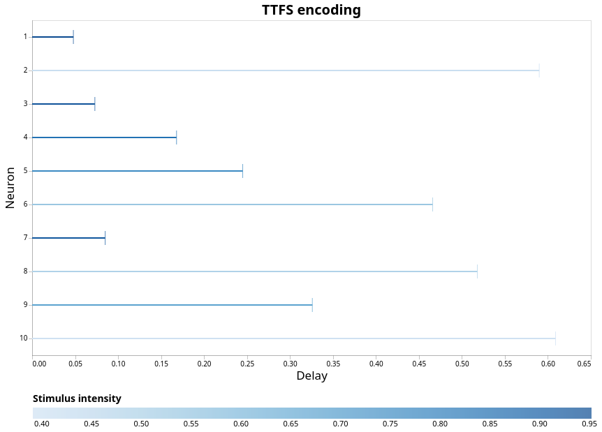
Figure 1:An example of time-to-first-spike (TTFS) encoding. The neurons encode (normalised) input stimuli, where larger values translate into shorter delays.
1.2.2.2Encoding with Gaussian Receptive Fields (GRFs)
The Gaussian Receptive Field (GRF) encoding scheme Bohte et al., 2002 is loosely modelled on the operating principle of the cochlea, where different sound frequencies are mapped to different physical locations. The GRF encoding mechanism is somewhat different to the ones introduced above in that it uses a population of neurons with overlapping receptive fields, whereby a real-valued input is encoded into a (potentially sparse) train of spikes with different delays.
In the GRF encoding scheme, each real-valued input variable is encoded by a population of equidistant neurons covering the interval of possible values that the variable can take. Each neuron is located at the peak of a Gaussian receptive field, and the distances between the peaks is chosen such that the receptive fields have significant overlap Fig. 3. For each input channel encoded by GRFs, the neurons should cover the entire range of values that the input for this channel could take.
The parameters ( and standard deviation ) of each Gaussian are chosen as follows:
Here, the parameter directly controls the width of the Gaussian receptive fields.
The input stimulus is mapped to the encoded interval . The vertical line originating at the point corresponding to the input stimulus (0.72 in Fig. 3) crosses the GRF for each encoding neuron. The vertical offset of the crossing point determines the delay for the corresponding neuron. An input value that is closer to the mean of a certain GRF would cause the neuron associated with that GRF to spike earlier. A threshold (denoted as here) can be used to sparsify the spike train, whereby if the delay is longer than the threshold, the neuron does not produce a spike.
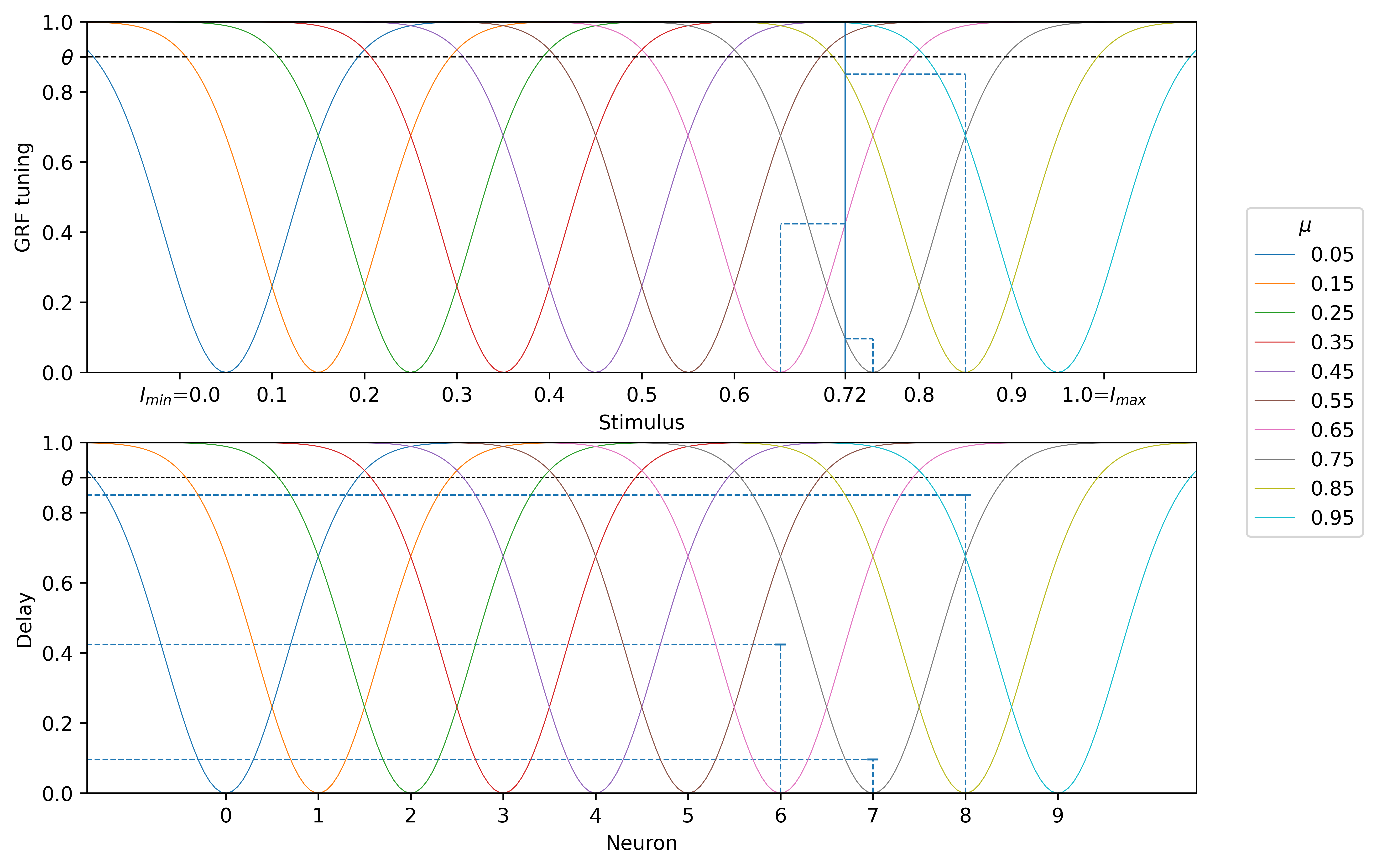
Figure 2:An example of encoding based on Gaussian Receptive Fields (GRF). Each input channel is encoded by a population of neurons with overlapping GRFs. This encoding resembles the encoding of sound in the cochlea, where different frequencies are encoded by populations of neurons in different physical locations along the cochlea.
Cite this chapter
Gaurav, Ramashish; Pedersen, Jens Egholm; Bogdan, Petrut (2026). Temporal Encoding. In Practical Spiking Neural Networks. Version 0.8. Open Neuromorphic. https://snnbook.net/topics/1_3_2_temp-enc
@incollection{snnbook2026-temp-enc,
  author    = {Gaurav, Ramashish and Pedersen, Jens Egholm and Bogdan, Petrut},
  title     = {{Temporal Encoding}},
  booktitle = {{Practical Spiking Neural Networks}},
  publisher = {Open Neuromorphic},
  year      = {2026},
  edition   = {Version 0.8},
  url       = {https://snnbook.net/topics/1_3_2_temp-enc},
}- Gollisch, T., & Meister, M. (2008). Rapid Neural Coding in the Retina with Relative Spike Latencies. Science, 319(5866), 1108–1111. 10.1126/science.1149639
- Bian, S., Donati, E., & Magno, M. (2024). Evaluation of Encoding Schemes on Ubiquitous Sensor Signal for Spiking Neural Network. IEEE Sensors Journal, 24(21), 35008–35018. 10.1109/JSEN.2024.3453927
- Eshraghian, J. K., Ward, M., Neftci, E. O., Wang, X., Lenz, G., Dwivedi, G., Bennamoun, M., Jeong, D. S., & Lu, W. D. (2023). Training Spiking Neural Networks Using Lessons From Deep Learning. Proceedings of the IEEE, 111(9), 1016–1054. 10.1109/JPROC.2023.3308088
- Bohte, S. M., Kok, J. N., & Poutré, H. L. (2002). Error-backpropagation in temporally encoded networks of spiking neurons. Neurocomputing, 48(1), 17–37.